
A tolerance stack up is the cumulative accumulation of dimensional variation across a chain of parts in an assembly — and the right starting method depends on your production context. For most stable, high-volume designs, start with RSS (root sum square) at 3σ. Use Monte Carlo when nonlinear geometry, non-normal distributions, or complex datum flows make linear RSS assumptions unreliable.
The core trade-off is conservatism versus cost. Worst-case guarantees assembly success but frequently overengineers parts. RSS and Monte Carlo reflect reality more accurately and can reduce manufacturing cost — but only when process capability is proven.
Quick decision checklist:
- Safety-critical interface or regulatory requirement → worst-case arithmetic
- Stable, high-volume production with known Cpk → RSS at 3σ
- Complex geometry, non-normal distributions, or nonlinear relationships → Monte Carlo
Your immediate next steps:
- Build the dimensional chain: identify every part and feature that contributes variation to the functional gap
- Assign nominal values, tolerance bands, and distributions to each contributor
- Run a quick RSS calculation in a spreadsheet to establish a baseline before committing to a method
Key Takeaways
Tolerance stack-up analysis is most effective when the method matches the production context: RSS for stable high-volume processes, worst-case for safety-critical interfaces, and Monte Carlo for complex geometry or non-normal distributions.
| Point | Details |
|---|---|
| Match method to context | Use worst-case for safety-critical or low-volume parts; RSS at 3σ for stable production; Monte Carlo for nonlinear or complex assemblies. |
| RSS vs. worst-case gap | For four contributors at ±0.06–0.08 mm, RSS predicts ±0.122 mm versus worst-case ±0.240 mm — a significant difference in required tolerance budget. |
| Process capability is required | Statistical tolerancing (RSS or Monte Carlo) is only valid when Cpk ≥ 1.0 and the process is monitored with SPC. |
| Model the datum flow chain | Datum mismatches between the stack model and the actual fixture or CMM program invalidate the analysis regardless of calculation method. |
| QA-Report for validation | QA-Report imports CMM data, auto-flags deviations, and tracks SPC history — giving engineers the process capability evidence that statistical tolerancing requires. |
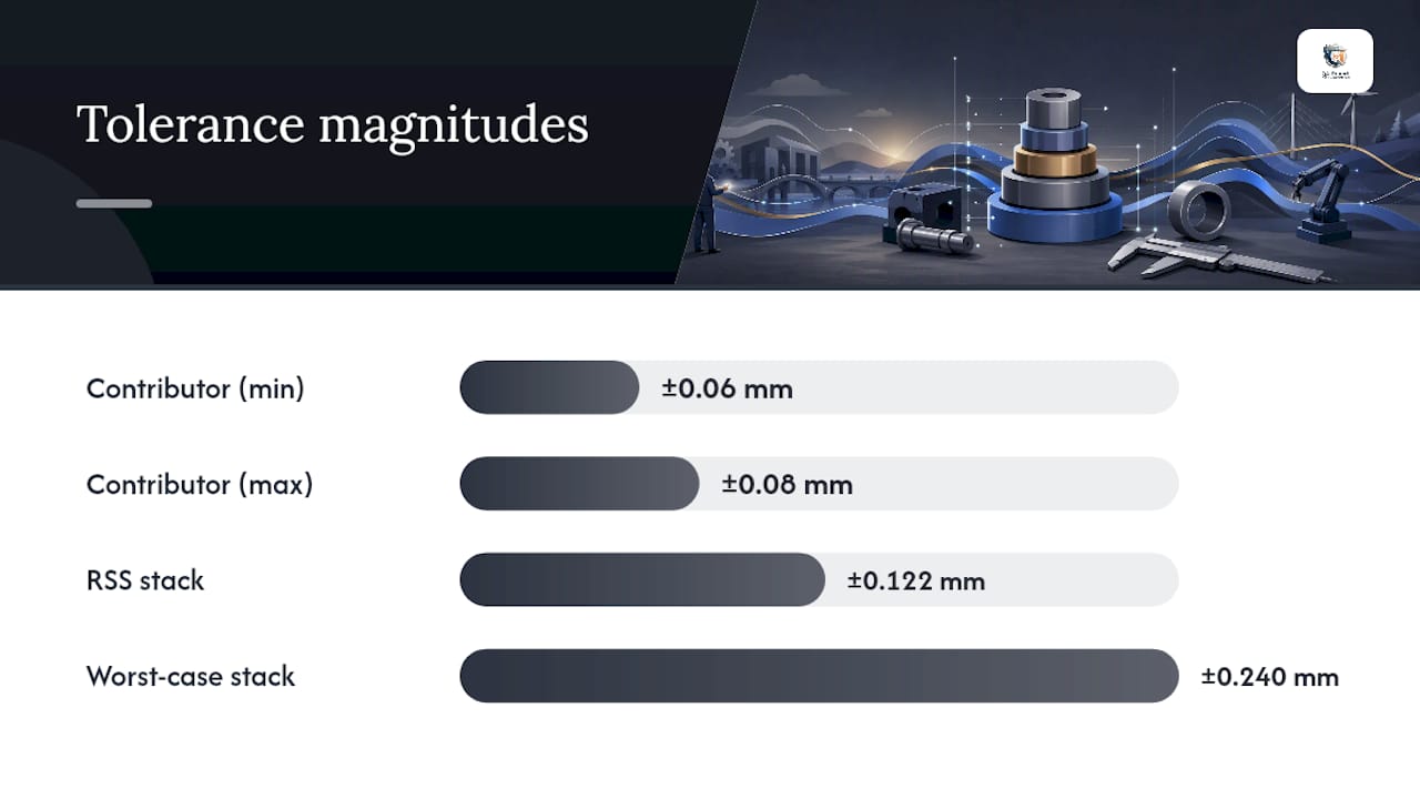
Table of Contents
- What is tolerance stack up, and why does it matter for your assembly?
- What are the core tolerance stack-up analysis methods?
- How do you perform a tolerance stack up? Step-by-step with a worked example
- How assembly models and datum flow chains affect your stack-up
- How to choose the right method and avoid costly stack-up mistakes
- Which tools should you use for tolerance stack-up analysis?
- Common errors in stack-up analysis and how to fix them
- Why Monte Carlo often reduces cost without sacrificing confidence
- An engineer's perspective on tolerance decisions in real projects
- How QA-Report closes the loop between stack-up predictions and inspection results
- Sources
What is tolerance stack up, and why does it matter for your assembly?
Even when every individual part passes inspection, the assembled system can still fail. That is the central problem tolerance stacking describes: dimensional variation accumulates across a chain of parts, and the summed result can exceed the functional requirement — producing interference, excessive clearance, misalignment, or preload loss.
Formally, a tolerance stack up models a dimensional chain (sometimes called a loop closure). You identify a functional requirement — a gap, a clearance, a contact force — and trace every dimension and tolerance that contributes to it. The loop closes when you return to the starting feature. The result is a predicted range for the functional parameter, not for any single part.
The distinction between part-level tolerance and assembly-level failure is where most problems originate. A shaft diameter held to ±0.05 mm and a bore held to ±0.05 mm are both conforming parts. But if the stack also includes a housing location tolerance of ±0.08 mm and a bearing seat runout of ±0.04 mm, the assembled clearance can vary far more than any individual drawing callout suggests.
Stack-up analysis applies most directly to design for assembly (DFA), first article inspection (FAI) planning, critical interface reviews, and high-volume production where yield loss from assembly failures is costly. It is less useful for single-part, non-mating features or for dimensions that have no functional relationship to adjacent components.
ASME Y14.5 is the governing standard for GD&T and dimensioning conventions in the United States, and it directly shapes how tolerances are modeled in a stack. Basic dimensions carry no tolerance themselves — tolerance comes from the associated geometric control. When you build a stack-up from a GD&T drawing, you must convert each geometric tolerance (position, runout, flatness) into its contribution to the dimensional chain, not simply read the ±dimension from a title block.
When sketching a dimensional chain, label each contributing dimension with its nominal value, its tolerance band, and its direction (positive or negative contribution to the functional gap). That sketch is your stack-up model — every feature that appears on it must be traceable to a drawing callout or a process specification.
What are the core tolerance stack-up analysis methods?
Five methods cover the practical range of assembly tolerance analysis. Each makes different assumptions about how variation combines, and each produces a different output.
Worst-case (arithmetic sum): Every tolerance is assumed to be at its extreme simultaneously. Total variation = Σ|T_i|. This guarantees 100% assembly success but is conservative — it treats a statistically rare event (all parts simultaneously at their worst) as the design condition.
RSS (root sum square / statistical): Treats individual tolerances as statistically independent and normally distributed. Total tolerance ≈ √(T₁² + T₂² + ... + Tₙ²). For three tolerances typically around ±0.10 mm, RSS predicts a notably smaller total variation than worst-case arithmetic, reflecting a reduced estimated assembly variation.
Monte Carlo simulation: Models actual distributions and geometry by running thousands of simulated assemblies drawn from input distributions. It produces a probability distribution of the functional output, including an estimated failure probability. Minitab's guidance recommends Monte Carlo when geometry or datum flow makes linear propagation inaccurate.
Linear propagation (sensitivity / Taylor series): Propagates variation through a mathematical model using partial derivatives (sensitivity coefficients). Accurate for mildly nonlinear systems; breaks down when the relationship between inputs and the functional output is strongly nonlinear.
Non-linear propagation (extended Taylor series / numerical integration): Extends the Taylor series to second-order terms or uses numerical integration to handle stronger nonlinearities. F. Scholz's technical report catalogs these methods alongside Monte Carlo and recommends integrating tolerancing through the design process rather than treating it as a late-stage check.
Method comparison
| Method | Conservatism | Realism / Statistical Accuracy | Data Input Requirements | Computational Complexity | Typical Outputs | When to Use |
|---|---|---|---|---|---|---|
| Worst-case (arithmetic) | Highest | Low — ignores probability | Nominal + tolerance band only | Minimal — hand calculation | Pass/fail margin; total variation | Safety-critical, low-volume, regulatory interfaces |
| RSS (statistical) | Moderate | Good for normal, independent inputs | Tolerance band; assumes 3σ process | Low — spreadsheet | Total σ, estimated yield at Cpk | Stable high-volume production with known Cpk |
| Monte Carlo | Low to moderate | Highest — models actual distributions | Full distributions per contributor | High — simulation software or script | Probability of failure, output distribution | Complex geometry, non-normal inputs, nonlinear stacks |
| Linear propagation | Moderate | Good for near-linear systems | Sensitivity coefficients + σ per input | Moderate — requires partial derivatives | Sensitivity ranking, total σ | Early design, sensitivity analysis |
| Non-linear propagation | Moderate | Better than linear for curved surfaces | Second-order derivatives or numerical model | High | More accurate σ for nonlinear systems | Assemblies with significant geometric nonlinearity |
Formula reference:
- Worst-case: T_total = Σ|T_i|
- RSS: T_total = √(ΣT_i²)
RSS assumes that tolerances are statistically independent and that each process is normally distributed, centered at nominal, and operating at approximately 3σ. When those assumptions do not hold — skewed distributions, correlated features, or off-center processes — Monte Carlo gives a more reliable answer.
How do you perform a tolerance stack up? Step-by-step with a worked example
Procedure
- Define the functional requirement. State the gap, clearance, or functional parameter you are analyzing and its specification limits (e.g., minimum clearance = 0.05 mm, maximum clearance = 0.40 mm).
- Build the dimensional chain. Trace every dimension from one side of the functional gap to the other, assigning a positive or negative sign based on direction of contribution.
- Assign nominals, tolerances, and distributions. Record the nominal value and bilateral tolerance for each contributor. For RSS or Monte Carlo, assign a distribution type (normal, uniform, or truncated normal) and convert the tolerance band to a standard deviation (σ = T/3 for a 3σ process).
- Select the analysis method. Apply the decision criteria from the method comparison above.
- Compute the result. Sum nominals for the mean gap; apply worst-case or RSS formula for the variation; or run the Monte Carlo simulation.
- Inspect the result. Compare the predicted variation to the specification limits. Calculate the predicted yield or failure probability.
- Iterate and reallocate. If the result fails, identify the largest contributors by their squared tolerance (for RSS) or absolute tolerance (for worst-case), tighten those first, or reduce the chain length.
Worked numeric example
Consider a simple 4-element linear stack: a shaft assembly where the functional requirement is a radial clearance between 0.05 mm and 0.45 mm.
Nominal clearance = (25.00 − 24.90) + (24.90 − 20.10) + (20.10 − 20.00) = 0.10 mm (simplified to the functional gap; actual loop closure gives the same result when signs are assigned correctly).
For this example, treat the functional gap as the sum of four contributing tolerances with the nominal gap = 0.20 mm.
Worst-case result: T_total = 0.08 + 0.05 + 0.05 + 0.06 = ±0.24 mm Predicted clearance range: 0.20 − 0.24 = −0.04 mm to 0.20 + 0.24 = 0.44 mm The lower bound is negative — interference is predicted at worst-case. This would flag a design concern.
RSS result (3σ): T_RSS = √(0.08² + 0.05² + 0.05² + 0.06²) = √(0.0064 + 0.0025 + 0.0025 + 0.0036) = √0.0150 ≈ ±0.122 mm Predicted clearance range: 0.20 − 0.122 = 0.078 mm to 0.20 + 0.122 = 0.322 mm Both bounds are within specification.
Monte Carlo summary (10,000 simulations, normal distributions at 3σ): Mean clearance ≈ 0.200 mm, σ_assembly ≈ 0.041 mm.
The worst-case result flags a potential interference that RSS and Monte Carlo show is statistically improbable. That gap between methods is where the cost decision lives: tighten all four tolerances to satisfy worst-case, or validate process capability and accept the RSS result.
A practical note on distribution conversion: when converting a bilateral tolerance to a standard deviation, σ = T/3 assumes the process is centered and operating at Cpk ≈ 1.0. If your supplier's Cpk is 1.33 or higher, you can use σ = T/4, which tightens the RSS prediction and increases predicted yield. For precision machining contexts, always confirm Cpk from actual SPC data before loosening tolerances based on RSS alone. Measurement error and thermal expansion are additional sources of variation that belong in the chain when they are significant relative to the tolerance band.
How assembly models and datum flow chains affect your stack-up
The accuracy of any stack-up depends on how faithfully the model reflects the actual assembly sequence and contact conditions. NIST's tolerancing research documents assembly models, datum flow chains, and a multilevel design-for-tolerance process that includes both linear and non-linear propagation methods — and the core message is that the model structure matters as much as the calculation method.
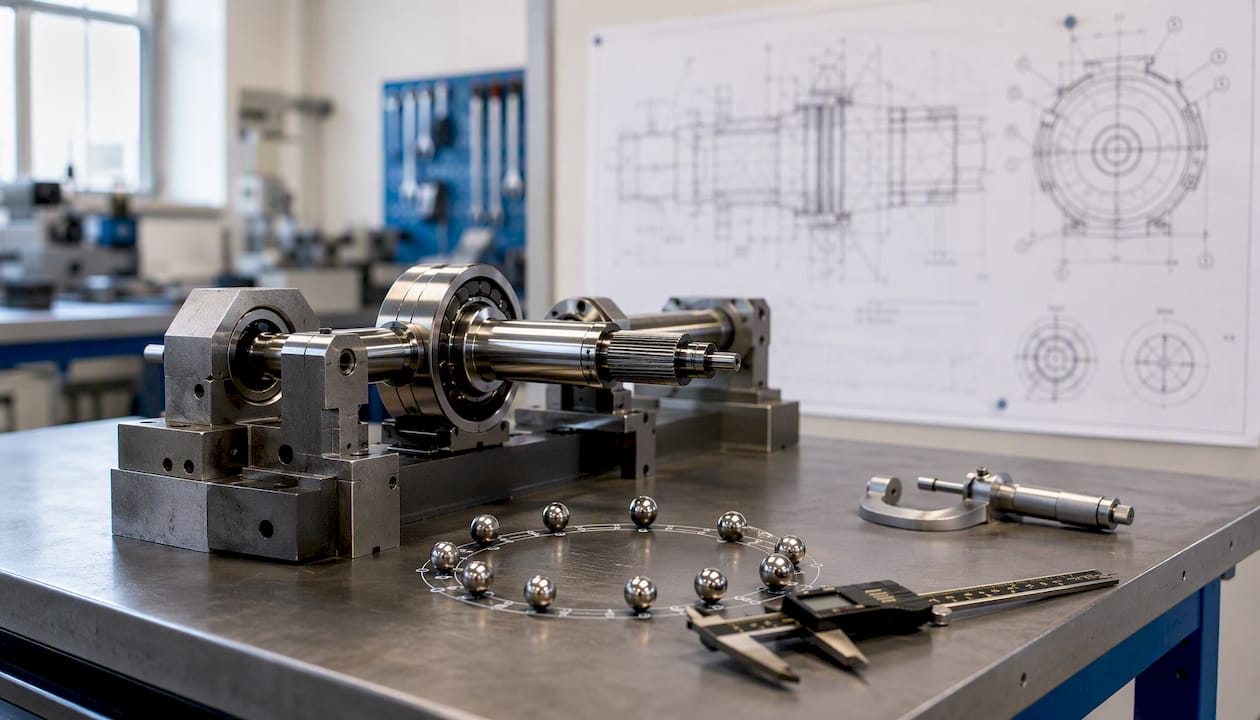
A datum flow chain traces how location and orientation are transferred from one part to the next through the assembly. In a shaft-bearing-housing assembly, the shaft is located by the bearing inner race, the inner race locates the outer race, and the outer race locates the housing. Each interface introduces a potential datum shift. If the housing datum is not the same feature used to machine the bore, a datum conversion tolerance enters the stack — and omitting it is one of the most common sources of field surprises.
Three assembly model types appear most frequently in practice. Hierarchical models represent assemblies as a tree of subassemblies, each contributing variation to the next level. Relational models capture the contact and constraint relationships between parts directly. Vector loop models close the dimensional chain algebraically, assigning a direction and magnitude to each contributor. For most linear assemblies, a vector loop in a spreadsheet is sufficient. For assemblies with angular features, curved surfaces, or multiple simultaneous constraints, a relational or 3D vector model is necessary.
Pro Tip: Before running any calculation, sketch the assembly sequence and mark every datum reference frame (DRF) transfer. A datum mismatch between design and fixturing can invalidate the entire stack-up, regardless of how carefully the math is done.
Common assembly modeling traps to check before finalizing your stack:
- Ignoring assembly sequence: the order parts are installed changes which features are constrained first and which float
- Omitting clamping deformation: fixturing forces can shift features by amounts comparable to the tolerance band in thin-walled or compliant parts
- Datum misalignment: using a different datum in the stack model than the one used in the fixture or CMM program
- Forgetting floating fastener clearance: bolt-hole position tolerances add directly to the stack when fasteners locate parts
- Missing subassembly variation: a pre-assembled subassembly carries its own accumulated variation into the next level
How to choose the right method and avoid costly stack-up mistakes
Method selection is not a matter of preference — it follows from the design context. Work through these criteria in order.
- Is the interface safety-critical or regulatory? If yes, use worst-case. No statistical argument overrides a regulatory requirement for 100% conformance at critical interfaces in aerospace (AS9100), medical devices (FDA 21 CFR Part 820), or automotive safety systems (IATF 16949).
- Is the manufacturing process stable and monitored? Statistical methods require a stable process with Cpk ≥ 1.0 and active SPC monitoring. Without that data, loosening tolerances based on RSS is a risk, not an engineering decision.
- What is the production volume? For low-volume or prototype runs, worst-case is practical and avoids the data requirements of statistical methods. For high-volume production, the cost savings from RSS or Monte Carlo justify the additional analysis effort.
- Is the geometry linear? If the functional output is a simple linear sum of contributing dimensions, RSS is appropriate. If the relationship involves angles, curved surfaces, or simultaneous constraints, use Monte Carlo or non-linear propagation.
- Do you have distribution data? Monte Carlo requires knowing (or assuming) the distribution shape for each contributor. If you only have tolerance bands, start with RSS and upgrade to Monte Carlo when inspection data is available.
Tolerance allocation priorities
When the initial stack-up fails, the corrective sequence matters. Tightening all tolerances equally is the most expensive solution and rarely necessary.
- Identify the top contributors by their squared tolerance (RSS) or absolute value (worst-case) — these are the features where tightening has the greatest leverage
- Tighten selectively on the highest contributors, checking cost-to-tighten against the manufacturing process for each feature
- Reduce chain length by redesigning to eliminate intermediate features or combining parts
- Add adjustment features (shims, set screws, eccentric pins) to absorb residual variation at assembly
- Use selective assembly for critical fits where tight tolerances are impractical on individual parts
- Switch to a tighter manufacturing process (grinding instead of turning, jig boring instead of conventional milling) for the one or two features that dominate the stack
Red flags that require worst-case analysis or further validation regardless of the method initially chosen: Cpk below 1.0 on any contributor, unknown or unqualified suppliers, first-run tooling without SPC history, regulatory interfaces, and assemblies where a single failure mode causes a safety event.
Which tools should you use for tolerance stack-up analysis?
The right tool depends on the design stage, the complexity of the assembly, and the data available. No single tool fits every situation.
Spreadsheets (Excel, Google Sheets): The fastest starting point for linear stacks. Build a column for nominal, tolerance, and σ; apply the RSS formula; read the result. Spreadsheets are appropriate for early-design feasibility checks and for communicating results to non-specialist stakeholders. They cannot handle 3D geometry or GD&T-aware datum conversions.
Python with NumPy/SciPy: The practical choice for Monte Carlo scripting when you need more than a spreadsheet but do not need a full commercial solver. A Monte Carlo loop in Python runs 10,000 to 100,000 simulations in seconds, accepts any distribution from SciPy's library, and produces a histogram of assembly outcomes. NumPy handles the random sampling; SciPy provides distribution fitting and statistical tests. This approach is well-suited to prototype validation and sensitivity studies.
MATLAB (MathWorks): Offers the same Monte Carlo capability as Python with stronger built-in statistical toolboxes and tighter integration with control and systems engineering workflows. MATLAB's Statistics and Machine Learning Toolbox supports distribution fitting, Monte Carlo, and sensitivity analysis in a single environment. It is the preferred choice in organizations that already use MATLAB for systems modeling.
CAD-integrated tolerance tools: SolidWorks TolAnalyst and Creo's EZ Tolerance Analysis Extension perform worst-case and statistical analysis directly on the CAD model, accounting for GD&T callouts and 3D geometry. PTC's documentation describes how these tools couple to the CAD model to handle datum conversions and geometric relationships that a spreadsheet cannot represent. They are the right choice when the critical dimension depends on orientation, non-parallel surfaces, or complex datum flow.
Commercial tolerancing suites:
- Sigmetrix CETOL 6σ: A dedicated 3D tolerance analysis platform that integrates with CATIA, Creo, and SolidWorks. CETOL performs sensitivity analysis, worst-case, RSS, and Monte Carlo on full 3D assemblies with GD&T-aware models. It is the standard tool in aerospace and automotive programs where the assembly model is complex and the analysis must be auditable.
- 3DCS (Dimensional Control Systems): A Monte Carlo-based 3D variation simulation tool that integrates with CATIA and other major CAD platforms. 3DCS models assembly sequence, fixture constraints, and part-to-part contact conditions, making it appropriate for body-in-white, powertrain, and other large assemblies where sequence and clamping effects are significant contributors.
Practical tool selection by design stage:
- Early design / feasibility: RSS in a spreadsheet, updated as the design matures
- Prototype validation: Monte Carlo in Python or MATLAB, using measured inspection data as input distributions
- Production release with complex GD&T: SolidWorks TolAnalyst or Creo EZ Tolerance Analysis for geometry-correct 3D stacks
- High-complexity production programs: Sigmetrix CETOL or 3DCS for auditable, GD&T-aware 3D Monte Carlo
For CMM-based inspection data that feeds back into the stack-up model, the key is mapping measured results to the dimensional chain contributors — so the simulation inputs reflect actual process performance rather than assumed distributions.
Common errors in stack-up analysis and how to fix them
Most stack-up failures trace back to a small set of recurring mistakes. Catching them before the parts are made is the entire point of the analysis.
Common errors:
- Ignoring assembly sequence: modeling the stack as if all parts float freely when the actual assembly constrains some features before others
- Omitting geometric tolerances: reading only ±dimensions from the title block and missing position, runout, or flatness callouts that contribute to the functional gap
- Assuming independence when features are correlated: a single machining setup that produces both a bore diameter and its location creates correlated errors that RSS underestimates
- Conflating tolerance band with standard deviation: using T directly as σ instead of σ = T/3 (or T/4 for a capable process) inflates the RSS result
- Forgetting systematic errors: fixture repeatability, CMM measurement uncertainty, and thermal expansion are real contributors that belong in the chain for tight-tolerance assemblies
Troubleshooting steps when a stack-up fails or produces unexpected results:
- Isolate the largest contributors by sorting squared tolerances (RSS) or absolute tolerances (worst-case) — the top two or three features typically account for most of the variation
- Run a short Monte Carlo test (even 1,000 simulations in a spreadsheet using RAND()) to check whether the RSS result is consistent with a simulated distribution
- Verify process capability with real SPC data from the supplier or shop floor before accepting any statistical tolerancing result; incoming inspection data is the most direct source
- Check the datum flow: confirm that the features in the stack model match the features used in the fixture and CMM program
- Add assembly adjustments (shims, set screws) or reduce chain length if tightening individual tolerances is cost-prohibitive
Corrective actions by cost and implementation time:
- Lowest cost, fastest: reallocate tolerances among existing features, tightening only the top contributors
- Moderate cost: add a shim or adjustment feature to absorb residual variation at assembly
- Higher cost: redesign mating features to reduce the number of contributors in the chain
- Highest cost, longest lead time: change the manufacturing process for a critical feature (e.g., switch from turning to grinding)
Why Monte Carlo often reduces cost without sacrificing confidence
The research case for probabilistic tolerancing is well-established. NIST's assembly tolerancing work documents that multilevel design-for-tolerance processes — integrating linear propagation, Monte Carlo, and datum flow chain analysis — produce more accurate predictions than worst-case arithmetic alone, particularly for assemblies with multiple contributors and complex geometry.
The cost argument is straightforward. Worst-case arithmetic assumes every part is simultaneously at its worst extreme — a condition that is statistically rare in any stable production process. Designing to that condition forces tighter tolerances than the process actually needs, which increases machining time, scrap rates, and inspection burden. Switching from worst-case to RSS or Monte Carlo can allow looser individual tolerances while maintaining an acceptable predicted yield — but only when process capability is proven and monitored.
The critical qualifier is process stability. Minitab's guidance is direct: statistical tolerancing requires a stable manufacturing process with adequate Cpk and active SPC monitoring. Without that foundation, loosening tolerances based on a Monte Carlo result is not a cost reduction — it is a yield risk. Real-time SPC software that tracks process capability continuously is the control that makes statistical tolerancing defensible.
F. Scholz's technical report on tolerance stack analysis methods reinforces this: the report catalogs linear propagation, extended Taylor series, numerical integration, and Monte Carlo as a progression of increasing accuracy and data requirements. The recommendation is to integrate tolerancing through the design process — not to apply it once at release — so that capability data informs the method choice at each stage.
The practical takeaway: use worst-case for feasibility and safety-critical interfaces, RSS for production allocation when Cpk is known, and Monte Carlo for final validation of complex assemblies. That sequence captures the cost benefit of statistical methods while preserving the safety margin where it matters.
An engineer's perspective on tolerance decisions in real projects
The gap between textbook stack-up analysis and shop-floor reality is wider than most design reviews acknowledge.
The most common failure mode is not a wrong formula — it is a wrong model. Engineers spend time debating worst-case versus RSS while the datum flow chain in the model does not match the actual fixture. The bearing seat is modeled as located from the housing centerline, but the fixture clamps on the outside diameter. That mismatch can introduce several times more variation than the tolerance difference between methods.
The second underestimated factor is measurement uncertainty. A CMM measurement of a bore diameter carries its own uncertainty — typically on the order of a few microns for a well-calibrated machine, but potentially much larger for complex GD&T features measured with a limited number of probe hits. When the tolerance band is tight, measurement uncertainty is not background noise; it is a contributor that belongs in the stack.
The practical approach that holds up across projects: use RSS for early tolerance allocation to get a realistic budget across contributors, reserve Monte Carlo for final validation of the two or three most critical interfaces, and require worst-case documentation for any interface that touches a safety or regulatory requirement. Document the stack-up in a controlled format that gets updated when tolerances change — a stack-up that was valid at design release can become invalid after a supplier change or a drawing revision.
How QA-Report closes the loop between stack-up predictions and inspection results
Predicting assembly variation is only half the work. The other half is confirming that the actual manufacturing process matches the distributions you assumed in the analysis.
QA-Report connects that loop directly. CMM data imports automatically into the platform, where the measurement wizard maps each measured dimension to its ballooned drawing callout and flags any out-of-tolerance deviation in real time. For tolerance validation workflows, that means you can compare actual measured variation against the σ values you used in your RSS or Monte Carlo model — and update the stack-up inputs when the process drifts.

Drawing ballooning with AI auto-numbering, GD&T support, and automated PDF report generation mean your inspection records satisfy AS9100, ISO 9001, and PPAP requirements without manual transcription. The integrated MES layer tracks batch and serial results over time, giving your team the SPC history that statistical tolerancing requires before you can responsibly loosen a tolerance. Start a free trial at Qa-report and import your first CMM dataset to see how measured results compare to your stack-up predictions.
Sources
Authoritative references for deeper study on assembly tolerance analysis and related standards:
- NISTIR 6223: Tolerancing and Assembly Models (excerpt)
- Understanding Tolerance Stack-Up Analysis: Building Confidence in Your Designs
- Tolerance Stacking: Calculation, Assembly Impact & Design Guide
- Tolerance Stack-Up Analysis — Worst Case vs RSS (Statistical) Methods - ficent design
- Tolerance Stack Analysis Methods (F. Scholz report)
- What is Tolerance Analysis? | PTC